
Investigating Stock Prediction with RNN
Investigating Stock Prediction with RNN
Overview
A recurrent neural network uses its internal state to process sequential inputs, which makes it great for time series data such as stock prices. LSTM has become the most popular technique on the Internet for machine learning stock prediction. Many claim to have astonishing accuracies. In this blog post, we will investigate the popular LSTM, long short-term memory, method for stock prediction.
We will construct in total three models using LSTM. The first one predicts one data point using multiple, which is the most popular technique and enjoys the most promising accuracy claims. The second model uses a different many-to-many technique for LTSM. Based on the previous two, we propose a hypothesis regarding the effectiveness of LSTM stock predictors and construct a third model to test our claim.
Here is a flow chart of our project.
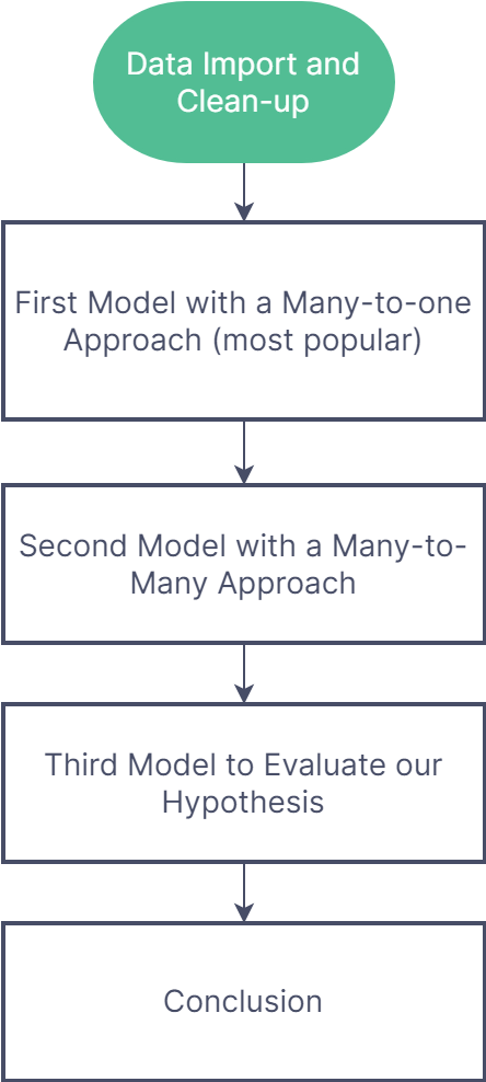
Here is the link to our GitHub repo. https://github.com/justinlaicy926/PIC16BProject
Data Import and Clean-up
#install yfinance in Colab
!pip install yfinance
#import the required libraries
import pandas as pd
import numpy as np
import keras
import tensorflow as tf
import plotly.graph_objects as go
from keras.preprocessing.sequence import TimeseriesGenerator
import math
import pandas_datareader as web
import numpy as np
import pandas as pd
from datetime import datetime
from sklearn.preprocessing import MinMaxScaler
import matplotlib.pyplot as plt
from pandas_datareader import data as pdr
import yfinance as yfin
from keras.models import Sequential
from keras.layers import LSTM, Dense, Dropout
import plotly.graph_objects as go
from sklearn.preprocessing import StandardScaler
from tensorflow.keras.optimizers import Adam
from plotly.io import write_html
import datetime as dt
from datetime import datetime
from keras.callbacks import ReduceLROnPlateau, ModelCheckpoint, TensorBoard
import model_helper
#yfinance api call to import data
yfin.pdr_override()
df = pdr.get_data_yahoo("^GSPC ^VIX", start="2002-01-01", end="2022-05-03")
[*********************100%***********************] 2 of 2 completed
#data cleanup
df["sp500"] = df["Adj Close"]["^GSPC"]
df["volume"] = df["Volume"]["^GSPC"]
df["vix"] = df["Adj Close"]["^VIX"]
df = df.reset_index()
df = df.drop(columns = ["Adj Close", "Volume"])
df = df.drop(columns = ["Close", "High", "Low", "Open"])
df.head()
/usr/local/lib/python3.7/dist-packages/pandas/core/generic.py:4150: PerformanceWarning: dropping on a non-lexsorted multi-index without a level parameter may impact performance.
obj = obj._drop_axis(labels, axis, level=level, errors=errors)
| Date | sp500 | volume | vix | |
|---|---|---|---|---|
| 0 | 2002-01-02 | 1154.670044 | 1171000000 | 22.709999 |
| 1 | 2002-01-03 | 1165.270020 | 1398900000 | 21.340000 |
| 2 | 2002-01-04 | 1172.510010 | 1513000000 | 20.450001 |
| 3 | 2002-01-07 | 1164.890015 | 1308300000 | 21.940001 |
| 4 | 2002-01-08 | 1160.709961 | 1258800000 | 21.830000 |
#replace with datetime
df['Date'] = pd.to_datetime(df['Date'])
df.set_axis(df['Date'], inplace=True)
#visualize our data
trace1 = go.Scatter(
x = df["Date"],
y = df["sp500"],
mode = 'lines',
name = 'SP500'
)
layout = go.Layout(
title = "S&P500 Index from 2002 to 2022",
xaxis = {'title' : "Date"},
yaxis = {'title' : "Close"}
)
fig = go.Figure(data=[trace1], layout=layout)
write_html(fig, "sp500.html")
#creates dataset for training and testing purposes
close_data = df['sp500'].values
close_data = close_data.reshape((-1,1))
split_percent = 0.80
split = int(split_percent*len(close_data))
#training and testing
close_train = close_data[:split]
close_test = close_data[split:]
date_train = df['Date'][:split]
date_test = df['Date'][split:]
#this will be the length for our RNN input
look_back = 20
#generate time series using this function
train_generator = TimeseriesGenerator(close_train, close_train, length=look_back, batch_size=20)
test_generator = TimeseriesGenerator(close_test, close_test, length=look_back, batch_size=1)
First Model with Many-to-One LSTM
Let’s make our first model with LSTM. We will be using the many-to-one method, i.e. input 20 data points of data and outputs 1 data point. We will be using the LSTM layers and dropout layers to construct our model.
#make our first model
model = Sequential()
#LSTM layer is the backbone of our RNN
model.add(
LSTM(50,
return_sequences=True,
activation='relu',
input_shape=(look_back,1))
)
model.add(
LSTM(50,
activation='relu',
input_shape=(look_back,1))
)
#dropout layer to prevent overfitting
model.add(Dropout(0.2))
model.add(Dense(1))
model.compile(optimizer='adam', loss='mse')
#fit our data with our model
model.fit_generator(train_generator, epochs=25, verbose=1)
Epoch 1/25
/usr/local/lib/python3.7/dist-packages/ipykernel_launcher.py:21: UserWarning: `Model.fit_generator` is deprecated and will be removed in a future version. Please use `Model.fit`, which supports generators.
204/204 [==============================] - 8s 26ms/step - loss: 307866.7188
Epoch 2/25
204/204 [==============================] - 4s 21ms/step - loss: 130283.4141
Epoch 3/25
204/204 [==============================] - 5s 26ms/step - loss: 92953.8828
Epoch 4/25
204/204 [==============================] - 4s 20ms/step - loss: 86772.0703
Epoch 5/25
204/204 [==============================] - 4s 20ms/step - loss: 83158.5938
Epoch 6/25
204/204 [==============================] - 4s 20ms/step - loss: 77838.5859
Epoch 7/25
204/204 [==============================] - 4s 20ms/step - loss: 77180.0312
Epoch 8/25
204/204 [==============================] - 4s 20ms/step - loss: 78002.9375
Epoch 9/25
204/204 [==============================] - 4s 20ms/step - loss: 86443.7188
Epoch 10/25
204/204 [==============================] - 4s 20ms/step - loss: 78251.7969
Epoch 11/25
204/204 [==============================] - 4s 21ms/step - loss: 74420.1328
Epoch 12/25
204/204 [==============================] - 4s 20ms/step - loss: 78686.7500
Epoch 13/25
204/204 [==============================] - 4s 21ms/step - loss: 75580.6406
Epoch 14/25
204/204 [==============================] - 4s 21ms/step - loss: 80284.8281
Epoch 15/25
204/204 [==============================] - 5s 22ms/step - loss: 76584.8359
Epoch 16/25
204/204 [==============================] - 4s 21ms/step - loss: 77448.7500
Epoch 17/25
204/204 [==============================] - 4s 21ms/step - loss: 74166.5781
Epoch 18/25
204/204 [==============================] - 4s 21ms/step - loss: 75540.6250
Epoch 19/25
204/204 [==============================] - 5s 26ms/step - loss: 74215.9531
Epoch 20/25
204/204 [==============================] - 4s 21ms/step - loss: 71973.0781
Epoch 21/25
204/204 [==============================] - 5s 23ms/step - loss: 76873.0234
Epoch 22/25
204/204 [==============================] - 4s 21ms/step - loss: 75014.7578
Epoch 23/25
204/204 [==============================] - 4s 21ms/step - loss: 77293.1016
Epoch 24/25
204/204 [==============================] - 4s 21ms/step - loss: 116743.6562
Epoch 25/25
204/204 [==============================] - 5s 23ms/step - loss: 138009.0938
<keras.callbacks.History at 0x7f1335e56510>
Now let’s see how our model predicts.
#make prediction
prediction = model.predict_generator(test_generator)
#reshape our prediction
close_train = close_train.reshape((-1))
close_test = close_test.reshape((-1))
prediction = prediction.reshape((-1))
#plots the three segments of data points, the training data, the predicted trend, and the actual price
trace1 = go.Scatter(
x = date_train,
y = close_train,
mode = 'lines',
name = 'Training Data'
)
trace2 = go.Scatter(
x = date_test,
y = prediction,
mode = 'lines',
name = 'Prediction'
)
trace3 = go.Scatter(
x = date_test,
y = close_test,
mode='lines',
name = 'Actual Price'
)
layout = go.Layout(
title = "SP500 Prediction",
xaxis = {'title' : "Date"},
yaxis = {'title' : "Close"}
)
fig = go.Figure(data=[trace1, trace2, trace3], layout=layout)
write_html(fig, "prediction1.html")
/usr/local/lib/python3.7/dist-packages/ipykernel_launcher.py:3: UserWarning: `Model.predict_generator` is deprecated and will be removed in a future version. Please use `Model.predict`, which supports generators.
This is separate from the ipykernel package so we can avoid doing imports until
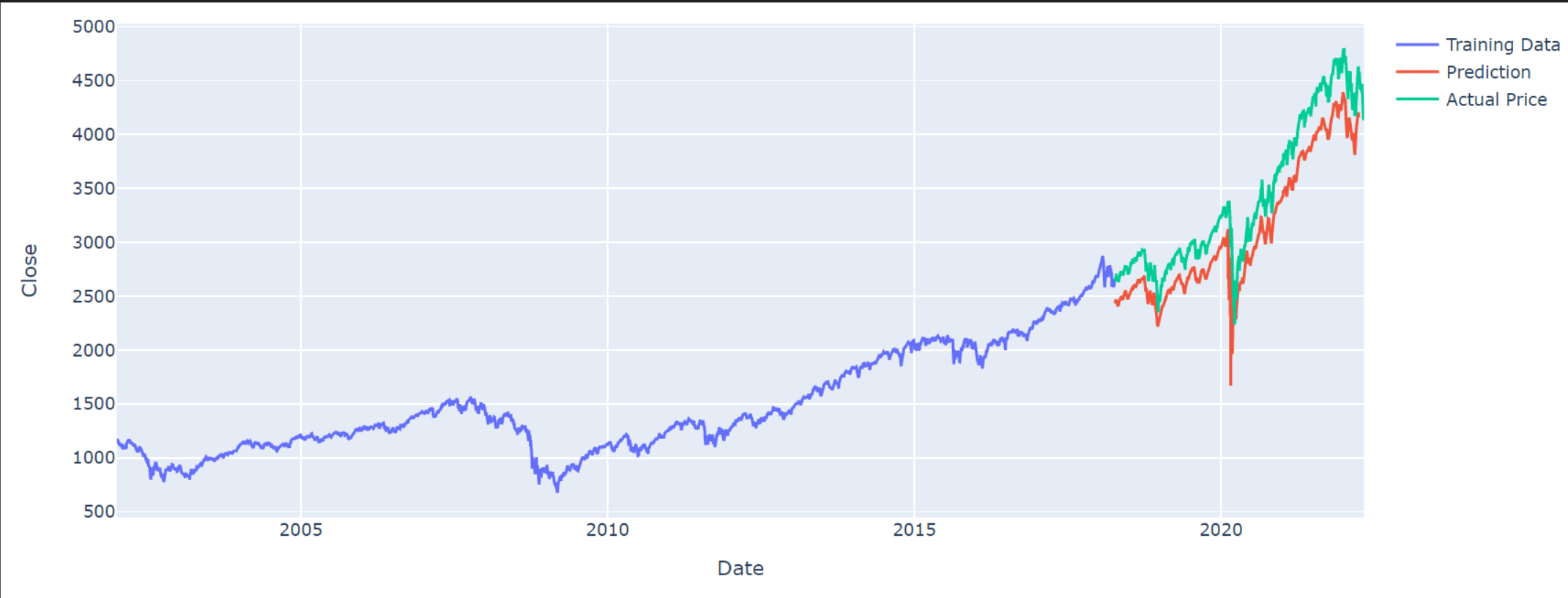
Our model is looking extremely promising. Our model has managed to accurately predict every major turning points in the stock market. If this is real, we would all be billionairs. But is there a catch? It almost looks too good to be true. Let’s see how it performs in the real world.
Making Prediction with Our First Model
We will predict 60 days into the future, 30 days of which is known data (to us, not to the model). Let’s see how our model performs.
#reshape our data
close_data = close_data.reshape((-1))
num_prediction = 60
forecast = predict(num_prediction, model)
forecast_dates = predict_dates(num_prediction)
#imports the actual price for these dates and cleans up
result = pdr.get_data_yahoo("^GSPC ^VIX", start="2022-05-02", end="2022-06-03")
result["sp500"] = result["Adj Close"]["^GSPC"]
result["voulme"] = result["Volume"]["^GSPC"]
result["vix"] = result["Adj Close"]["^VIX"]
result = result.reset_index()
result = result.drop(columns = ["Adj Close", "Volume"])
result = result.drop(columns = ["Close", "High", "Low", "Open"])
result['Date'] = pd.to_datetime(result['Date'])
result.set_axis(result['Date'], inplace=True)
close_data = result['sp500'].values
close_data = close_data.reshape((-1,1))
actual_date = result['Date']
actual_close = close_data
[*********************100%***********************] 2 of 2 completed
/usr/local/lib/python3.7/dist-packages/pandas/core/generic.py:4150: PerformanceWarning:
dropping on a non-lexsorted multi-index without a level parameter may impact performance.
#plots the real-world prediction
trace1 = go.Scatter(
x = forecast_dates,
y = forecast,
mode = 'lines',
name = 'Data'
)
trace2 = go.Scatter(
x = result['Date'],
y = result['sp500'].values,
mode = 'lines',
name = 'Actual Price'
)
layout = go.Layout(
title = "SP500 Prediction",
xaxis = {'title' : "Date"},
yaxis = {'title' : "Close"}
)
fig = go.Figure(data=[trace1, trace2], layout=layout)
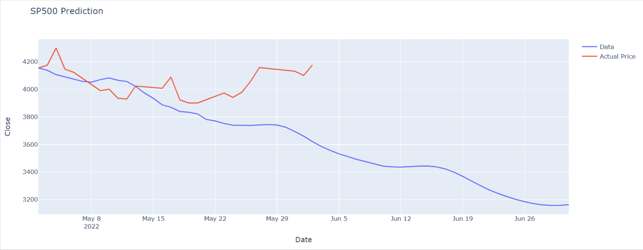
With just two months of prediction, we are seeing a significant deviation from the actual price trend. Our model tells us that SP500 will continue tanking for two months, with no significant pullbacks. This is highly unlikely based on experience. The actual price trend, however, is much more reasonable.
Second Model with Many-to-Many RNN
We saw some significant drawbacks with our first model in the real world. It is shocking how good it is with test cases until it performs against unseen data. In this section, we will try to explain this discrepancy with our second model using the many-to-many method.
Instead of feeding our model with 20 data points and extracting one prediction, we will be feeding it with multiple data points and extracting a trend line into the future.
#Data import and cleanup
dataset_train = pd.read_csv('^NDX.csv')
cols = list(dataset_train)[1:]
datelist_train = list(dataset_train["Date"])
datelist_train = [dt.datetime.strptime(date, '%Y-%m-%d').date() for date in datelist_train]
training_set = dataset_train.values
#feature scaling using StandardScalar
sc = StandardScaler()
training_set_scaled = sc.fit_transform(training_set)
#shapes our data
sc_predict = StandardScaler()
sc_predict.fit_transform(training_set[:, 0:1])
array([[-0.703329 ],
[-0.69582021],
[-0.6775205 ],
...,
[ 2.4043269 ],
[ 2.47115722],
[ 2.476595 ]])
For consistency’s sake, we will look into the future for 60 days just like before. But instead of looking back for 20 days, we will likely need more data points. Let’s use 90 days of trading data to predict the next 60 days of prices.
#create our training data set
X_train = []
y_train = []
#predict 60 days with 90 days
n_future = 60
n_past = 90
for i in range(n_past, len(training_set_scaled) - n_future +1):
X_train.append(training_set_scaled[i - n_past:i, 0:dataset_train.shape[1] - 1])
y_train.append(training_set_scaled[i + n_future - 1:i + n_future, 0])
X_train, y_train = np.array(X_train), np.array(y_train)
#Similar deal, sequential model with 2 LSTM models and one dropout
model = Sequential()
model.add(LSTM(units=64,
return_sequences=True,
input_shape=(n_past, dataset_train.shape[1]-1)))
model.add(LSTM(units=10,
return_sequences=False))
model.add(Dropout(0.20))
model.add(Dense(units=1, activation='linear'))
#compile the model
model.compile(optimizer = Adam(learning_rate=0.01), loss='mean_squared_error')
#fit the model
model.fit(X_train, y_train, epochs=20)
#makes the list for prediction
datelist_future = pd.date_range(datelist_train[-1], periods=n_future, freq='1d').tolist()
#makes the list of dates
datelist_future_ = []
for this_timestamp in datelist_future:
datelist_future_.append(this_timestamp.date())
#makes the prediction
predictions_future = model.predict(X_train[-n_future:])
predictions_train = model.predict(X_train[n_past:])
#cleans up the data for visualization
y_pred_future = sc_predict.inverse_transform(predictions_future)
y_pred_train = sc_predict.inverse_transform(predictions_train)
PREDICTIONS_FUTURE = pd.DataFrame(y_pred_future, columns=['Open']).set_index(pd.Series(datelist_future))
PREDICTION_TRAIN = pd.DataFrame(y_pred_train, columns=['Open']).set_index(pd.Series(datelist_train[2 * n_past + n_future -1:]))
PREDICTION_TRAIN.index = PREDICTION_TRAIN.index.to_series()
dataset_train = pd.DataFrame(dataset_train, columns=cols)
dataset_train.index = datelist_train
dataset_train.index = pd.to_datetime(dataset_train.index)
START_DATE_FOR_PLOTTING = '2012-05-01'
trace1 = go.Scatter(
x = PREDICTIONS_FUTURE.index,
y = PREDICTIONS_FUTURE['Open'],
mode = 'lines',
name = 'Predicted Stock Price'
)
trace2 = go.Scatter(
x = PREDICTION_TRAIN.loc[START_DATE_FOR_PLOTTING:].index,
y = PREDICTION_TRAIN.loc[START_DATE_FOR_PLOTTING:]['Open'],
mode = 'lines',
name = 'Training Predictions'
)
trace3 = go.Scatter(
x = dataset_train.loc[START_DATE_FOR_PLOTTING:].index,
y = dataset_train.loc[START_DATE_FOR_PLOTTING:]['Open'],
mode = 'lines',
name = 'Actual Stock Prices'
)
layout = go.Layout(
title = "NQ100 Prediction",
xaxis = {'title' : "Date"},
yaxis = {'title' : "Close"}
)
fig = go.Figure(data=[trace1, trace2, trace3], layout=layout)
write_html(fig, "prediction3.html")
This looks nothing like before. Our model has completely failed to predict the upward rally beginning march 2020. In fact, it has failed to predict any breakage of establish trend. It appears it is trained to stick to existing trends in an effort to maximize accuracy. This model is useless in the real world.
But what causes the stark difference between our first and second model? In a many-to-many model tested against seen data, the model is always tasked with predicting the next day. It is easy to guess the next data point as stock prices are relatively continuous, and our model can always guess some number close. Since we are testing with seen data, any miscalculation does not add up. But when facing unseen prediction, our model fails. The second model is a clear demonstration of how our model fails to predict any change in price trends.
Third Model
We hypothesize that our RNN model is simply adhering to the most dominant trend. Instead of prediction based on identifying trends and patterns, which was expected from RNN, it is acting more of a regression role. Thus, we decide to conduct a third model based on data points from March 2020 to present day.
During this time period, aggresive monetary and fiscal policies reshaped market. The resulting stock market performance deviated from the pre-established trends for over a decade. If our hypothesis is true, our third model will guess the stock market will stcik to a never ending upward rally.
Model 3 is exactly the same as our previous model, except trained with localized data.
yfin.pdr_override()
df = pdr.get_data_yahoo("^GSPC ^VIX", start="2020-03-15", end="2022-06-05")
df = df.reset_index()
[*********************100%***********************] 2 of 2 completed
df.head()
dataset_train = pd.concat([df['Date'],df['Open']['^GSPC'],df['High']['^GSPC'],df['Low']['^GSPC'],df['Close']['^GSPC'],df['Adj Close']['^GSPC'],df['Volume']['^GSPC']],axis=1)
dataset_train.columns=["Date","Open","High","Low","Close","Adj Close","Volume"]
cols = list(dataset_train)[1:]
datelist_train = list(dataset_train['Date'])
datelist_train = [dt.datetime.strptime(str(date), '%Y-%m-%d %H:%M:%S').date() for date in datelist_train]
training_set = dataset_train[cols].astype(str)
training_set = training_set.astype(float)
training_set = training_set.values
training_set
array([[2.50859009e+03, 2.56297998e+03, 2.38093994e+03, 2.38612988e+03,
2.38612988e+03, 7.78154000e+09],
[2.42565991e+03, 2.55392993e+03, 2.36704004e+03, 2.52918994e+03,
2.52918994e+03, 8.35850000e+09],
[2.43650000e+03, 2.45357007e+03, 2.28052002e+03, 2.39810010e+03,
2.39810010e+03, 8.75578000e+09],
...,
[4.14977979e+03, 4.16654004e+03, 4.07385010e+03, 4.10122998e+03,
4.10122998e+03, 4.14571000e+09],
[4.09540991e+03, 4.17750977e+03, 4.07437012e+03, 4.17681982e+03,
4.17681982e+03, 3.60493000e+09],
[4.13756982e+03, 4.14266992e+03, 4.09866992e+03, 4.10854004e+03,
4.10854004e+03, 3.10708000e+09]])
sc = StandardScaler()
training_set_scaled = sc.fit_transform(training_set)
sc_predict = StandardScaler()
sc_predict.fit_transform(training_set[:, 0:1])
# Creating a data structure with 90 timestamps and 1 output
X_train = []
y_train = []
n_future = 60
n_past = 90
for i in range(n_past, len(training_set_scaled) - n_future +1):
X_train.append(training_set_scaled[i - n_past:i, 0:dataset_train.shape[1] - 1])
y_train.append(training_set_scaled[i + n_future - 1:i + n_future, 0])
X_train, y_train = np.array(X_train), np.array(y_train)
print('X_train shape == {}.'.format(X_train.shape))
print('y_train shape == {}.'.format(y_train.shape))
X_train shape == (412, 90, 6).
y_train shape == (412, 1).
model = Sequential()
model.add(LSTM(units=64, return_sequences=True, input_shape=(n_past, dataset_train.shape[1]-1)))
model.add(LSTM(units=10, return_sequences=False))
model.add(Dropout(0.25))
model.add(Dense(units=1, activation='linear'))
model.compile(optimizer = Adam(learning_rate=0.01), loss='mean_squared_error')
rlr = ReduceLROnPlateau(monitor='val_loss', factor=0.5, patience=10, verbose=1)
mcp = ModelCheckpoint(filepath='weights.h5', monitor='val_loss', verbose=1, save_best_only=True, save_weights_only=True)
tb = TensorBoard('logs')
history = model.fit(X_train, y_train, shuffle=True, epochs=30, callbacks=[rlr, mcp, tb], validation_split=0.2, verbose=1, batch_size=256)
datelist_future = pd.date_range(datelist_train[-1], periods=n_future, freq='1d').tolist()
datelist_future_ = []
for this_timestamp in datelist_future:
datelist_future_.append(this_timestamp.date())
predictions_future = model.predict(X_train[-n_future:])
predictions_train = model.predict(X_train[n_past:])
y_pred_future = sc_predict.inverse_transform(predictions_future)
y_pred_train = sc_predict.inverse_transform(predictions_train)
PREDICTIONS_FUTURE = pd.DataFrame(y_pred_future, columns=['Open']).set_index(pd.Series(datelist_future))
PREDICTION_TRAIN = pd.DataFrame(y_pred_train, columns=['Open']).set_index(pd.Series(datelist_train[2 * n_past + n_future -1:]))
# Convert <datetime.date> to <Timestamp> for PREDCITION_TRAIN
PREDICTION_TRAIN.index = PREDICTION_TRAIN.index.to_series().apply(datetime_to_timestamp)
PREDICTION_TRAIN
trace1 = go.Scatter(
x = PREDICTIONS_FUTURE.index,
y = PREDICTIONS_FUTURE['Open'],
mode = 'lines',
name = 'Predicted Stock Price'
)
trace2 = go.Scatter(
x = PREDICTION_TRAIN.index,
y = PREDICTION_TRAIN['Open'],
mode = 'lines',
name = 'Training Predictions'
)
trace3 = go.Scatter(
x = dataset_train['Date'],
y = dataset_train['Open'],
mode = 'lines',
name = 'Actual Stock Prices'
)
layout = go.Layout(
title = "NQ100 Prediction",
xaxis = {'title' : "Date"},
yaxis = {'title' : "Close"}
)
fig = go.Figure(data=[trace1, trace2, trace3], layout=layout)
fig.show()
write_html(fig, "prediction4.html")
It appears our model has performed exactly as we have hypothesized. In other words, our use of RNN fails to predict significant trend movements to enable profitable trades. Instead of prediction, our model excels at regression.
Conclusion
Our many-to-many model shows the real-world usefulness, or the lack thereof, of modelling stock prices using RNN. We remain skeptical of technical analysis doctrince based on price trend analysis.
Despite our search for a reliable technical analysis RNN model has failed, it is insufficient to conclude the merit of all technical analysis methods. More in-depth experimentation is needed.